Author: Andrew

A lot of the early development of quantum mechanics focused on the hydrogen atom. Fortunately, the hydrogen atoms that are around today are just as good as the ones from the 1910’s and furthermore we’ve got the benefit of hindsight and improved instruments to help us. So let’s take a look at what raw experimental data we can get from hydrogen and use that to trace the development of ideas in quantum mechanics.

Back in 1740’s, lots of people were messing around with static electricity. For example, the first capacitor (the Leyden jar) was invented in 1745, allowing people to store larger amounts of electrical energy. Anyone playing around with electricity – even just rubbing your shoes across a carpet – is familiar with the fact that electricity can jump across small distances of air. In 1749, Abbe Nollet was experimenting with “electrical eggs” which was a glass globe with some of the air pumped out, with two wires poking into it. Pumping the air out allowed longer sparks, apparently giving enough light to read by at night. (Aside: one of these eggs featured in a painting from around 1820 by Paul Lelong). a video of someone with a hydrogen-filled tube so we don’t all have to actually buy one.

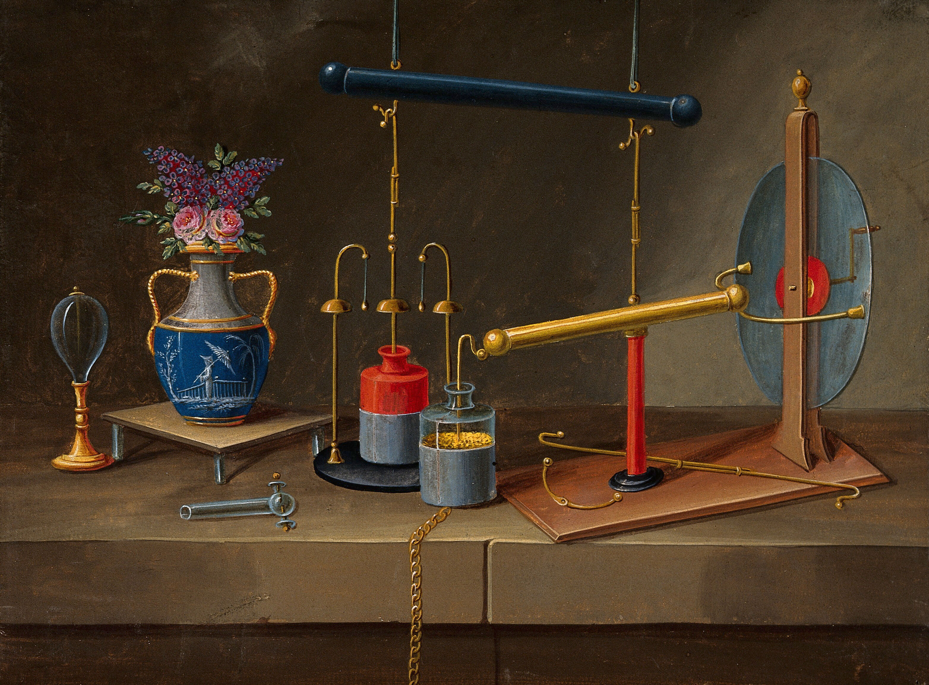
By passing the light through a diffraction grating (first made in 1785, although natural diffraction gratings such as feathers were in use by then) the different wavelengths of light get separated out to different angles. When we do this with the reddish glow of the hydrogen tube, it separates out into three lines – a red line, a cyan line, and a violet line. Although many people were using diffraction gratings to look at light (often sunlight) it was Ångström who took the important step of quantifying the different colours of light in terms of their wavelength (Kirchoff and Bunsen used a scale specific to their particular instrument). This accurately quantified data, published in 1868 in Ångström’s book was crucial. Although Ångström’s instrument allowed him to make accurate measurements of lines, he was still just using his eyes and therefore could only measure lines in the visible part of the spectrum (380 to 740nm). The three lines visible in the youtube video are at 656nm (red), 486nm (cyan), 434nm (blue) and there’s a 4th line at 410nm that doesn’t really show up in the video.

These four numbers are our first clues, little bits of evidence about what’s going on inside hydrogen. But the next breakthrough came apparently from mere pattern matching. In 1885 Balmer (an elderly school teacher) spotted that those numbers have a pattern to them. If you take the series n^2/(n^2-2^2) for n=3,4,5… and multiply it by 364.5nm then the 4 hydrogen lines pop out (eg. for n=3 we have 365.5 * 9/(9-4) = 656nm and for n=6 we have 365.5 * 36/32 = 410nm). Alluringly, that pattern suggests that there might be more than just four lines. For n=7 it predicts 396.9nm which is just into the ultraviolet range. As n gets bigger, the lines bunch up as they approach the “magic constant” 365.5nm.

We now know those visible lines are caused when the sole electron in a hydrogen atom transitions to the second-lowest energy state. Why second lowest and not lowest? Jumping all the way to the lowest gives off photons with more energy, so they are higher frequency aka shorter wavelengths and are all in the ultraviolet range that we can’t see with our eyes.

Balmer produced his formula in 1885, and it was a while until Lyman went looking for more lines in the ultraviolet range in 1906 – finding lines starting at 121nm then bunching down to 91.175nm – and we now know these are jumps down to the lowest energy level. Similarly, Paschen found another group of lines in the infrared range in 1908, then Brackett in 1922, Pfund in 1924, Humphreys in 1953 – as better instruments allowed them to detect those non-visible.

Back in 1888, three years after Balmers discovery, Rydberg was trying to explain the spectral lines from various different elements and came up with a more general formula, of which Balmer’s was just a special case. Rydberg’s formula predicted the existence (and the wavelength) of all these above groups of spectral lines. However, neither Rydberg or Balmer suggested any physical basis for their formula – they were just noting a pattern.

To recap: so far we have collected a dataset consisting of the wavelengths of various spectral lines that are present in the visible, ultraviolet and infrared portions of the spectrum.

In 1887, Michelson and Morley (using the same apparatus they used for their famous ether experiments) were able to establish that the red hydrogen line ‘must actually be a double line’. Nobody had spotted this before, because it needed the super-accurate interference approach used by Michelson and Morley as opposed to just looking at the results of a diffraction grating directly. So now we start to have an additional layer of detail – many of the lines we thought were “lines” turn out to be collections of very close together lines.

In order to learn about how something works, it’s a good idea to prod it and poke it to see if you get a reaction. This was what Zeeman did in 1896 – subjecting a light source (sodium in kitchen salt placed in a bunsen burner flame) to a strong magnetic field. He found that turning on the magnet makes the spectral lines two or three times wider. The next year, having improved his setup, he was able to observe splitting of the lines of cadmium. This indicates that whatever process is involved in generating the spectral lines is influenced by magnetic fields, in a way that separates some lines into two, some into three, and some don’t split at all.

Another kind of atomic prodding happened in 1913 when Stark did an experiment using strong electric fields rather than magnetic fields. This also caused shifting and splitting of spectral lines. We now know that the electric field alters the relative position of the nucleus and electrons, but bear in mind that the Rutherford goil foil experiment which first suggested that atoms consist of a dense nucleus and orbiting electrons was published in 1913 and so even the idea of a ‘nucleus’ was very fresh at that time.

Finally, it had been known since 1690 that light exhibited polarization. Faraday had shown that magnets can affect the polarization of light, and ultimately this had been explained by Maxwell in terms of the direction of the electric field. When Zeeman had split spectral lines using magnetic field, he noticed the magnetic field affected polarization too.

So that concludes our collection of raw experimental data that was available to the founders of quantum mechanics. We have accurate measurements of the wavelength of spectral lines for various substances – hydrogen, sodium etc – and the knowledge that some lines are doublets or triplets and those can be shifted by both electric and magnetic fields. Some lines are more intense than others.

It’s interesting to note what isn’t on that list. The lines don’t move around with changes in temperature. They do change if the light source is moving away from you at constant velocity, but this was understood to be the doppler effect due to the wave nature of light rather than any effect on the light-generating process itself. I don’t know if anyone tried continuously accelerating the light source, eg. in a circle, to see if that changed the lines, or to see if nearby massive objects had any impact.

I was walking north in London. I was definitely walking north. My phone map showed I was going north. The road signs pointed straight ahead to go to Kings Cross, which was to the north. I knew I going north. But, in a post-apocalyptic way, I also like trying to navigate by using the sun. It was afternoon. The sun would be setting in the west. I was heading north. Shadows would stretch out to my right. I looked at the shadows on the ground. They were stretching out to the left. Left, not right. Wrong. I stopped dead, now completely unsure which direction I was going and what part of my reasoning chain was broken.

It took me a while, but I figured it out. There were tall buildings to my left blocking the direct sun. On my right was tall glass-fronted offices. The windows were bouncing sunlight from up high down onto the pavement. From the “wrong” direction!

Moral of the story: don’t trust the sun!

My two interests of air crash investigations and financial systems are coinciding today as I read through the Coop Bank annual results. Unlike RBS’s decline in 2008, this isn’t a dramatic story of poorly understood risk lurking behind complex financial instrument, it’s a bit more straightforward. But, since I spent some time picking through the numbers I thought I’d capture it for posterity.

A traditional high-street bank makes money from loans because customers have to pay interest on their mortgages and car loans, hence banks consider loans to be assets. The money which you or I have in our current or instant-access saving accounts, “demand deposits”, are liabilities of the bank. The bank pays out interest to savers. Unsurprisingly, the interest rate on loans is higher than what the bank pays to savers, and the difference (called “net interest income”) is income for the bank which ideally helps increase the banks equity (ie. money owned by the bank, which shareholders have claims on).

At first glance, Coop Bank are doing fine here. They have £15.3bn of loans to people (14.8bn) and businesses (0.4bn). They have £22.1bn of customer deposits [page 16], spread fairly evenly between current accounts, instant savings accounts, term savings accounts and ISAs, being a mixture of individuals (£19.4bn) and companies (£2.7bn). A quick check of their website shows they pay savers around 0.25%, and mortgage rates around something like 3%, which directly gets you to their “net interest income” of £394m from their high-street (aka “retail operations”). So that’s a big bunch of money coming in the door, good news!

(They used to be big into commercial property loans, but by 2014 their £1650m of loans included about £900m which were defaulting, and they sold off the rest and got out of that business)

But every business has day-to-day costs, like rent and staff salaries to pay. Staff costs were £187m which sounds like a lot of money, but a UK-wide bank has a lot of staff – 4266 [page 33] of which 3748 were fulltime and 1018 part-time. That’s an average of £43k each, but it’s not spread evenly – the four executive directors got £4172k between them [page 92], and the eleven non-exec directors got £1052k between them [page 95]. In addition, they paid £121m on contractors [page 178]. So, total staff costs were £300m. Hmm, now that £394m income isn’t looking so peachy. We’ve only got £94m left – let’s hope there’s nothing else we have to pay for.

Oops, forgot about the creaking IT infrastructure! The old IT setup was pretty bad it seems. The bank themselves warned investors in 2015 that “the Bank does not
currently have a proven end-to-end disaster recovery capability, especially in the case of a
mainframe failure or a significant data centre outage.” (page 75). The FCA (Financial Conduct Authority) who regulate banks and check that they are at least meeting some basic minimum standards told the Coop Bank in 2015 that they were in breach of those basic standards. So, they came up with a cunning plan to get off their clunky mainframes and onto a whizzy IBM “managed service platform” which, one would hope, is much shinier and has a working and tested backup solution. All of this “remediation” work wasn’t cheap though, clocking in at £141m for the year. The good news is that the FCA are all happy again and it should be a one-off cost, but we’re looking at loss overall for the year of £47m.

But we’re not done yet! We also have some “strategic” projects on the go, which managed to burn £134m [page 19]. A while back, Coop decided to “outsource” its retail mortgage business to Capita, and then spent a lot of time bickering with them, before finally making up this year. Nonetheless, a planned “transformation” of IT systems is getting canned, the demise of which is somehow costing the bank £82m! At the more sensible end, £10m went into “digital” projects, which I assume includes their shiny new mobile app [page 12]. But all in all, those “strategic” projects means we’re now up to a £181m loss.

Only one more big thing to go. Back in 2009, Coop Bank merged/acquired Britannia Building Society, gaining about £4bn of assets in the form of risky commercial property loans, and some liabilities. Those liabilities included IOUs known as Leek Notes which Britannia had issued to get money in the short-term. When Coop acquired Britannia, there was some accountancy sleight of hand done to make the liability look smaller [page 26 in Kelly Review] but nonetheless a £100 IOU still has to ultimately be paid back with £100, and so now Coop Bank is drudging through the reality of a paying back (aka “unwinding”, gotta love the euphemisms) a larger-then-expected liability. In 2016, that was to the tune of £180m.

So now we’re up to a £361m loss. Chuck in a few more projects like EU Payment Directives, some “organizational design changes” which cost £20m and you get to a final overall loss for the year of £477m.

Now, in the same way that I (as a person) can have money that I own in my pocket, Banks can have money that they (as a company) own – which is their equity. In good times, some of that equity gets paid out to shareholders as a dividend, and some is retained within the company to fund future growth. But in bad times, that equity is eroded by losses. Coop Bank started the year with about £1100m of (tier 1) equity, and the £400m loss has chopped that down to £700m. If you’re losing £400m in a year, £700m doesn’t look like a lot of runway and that’s why they’re trying to sell the business or bit of it, or raise equity by converting bonds to shares or issuing bonds.

Like any business, you’ve got to have more assets than liabilities otherwise your creditors can have you declared insolvent. And Coop Bank certainly has more assets than liabilities. But the loans which make up part of the banks assets are fairly illiquid, meaning they can’t be readily turned into cash. Furthermore, they’re somewhat risky since the borrower might run away and default on the loan. So, in order to be able to soak up defaulting loans and have enough money around to people to withdraw their deposits on demand, banks need to have a certain level of equity in proportion to their loans. You can either look at straight equity/assets, aka leverage ratio, which is 2.6% for Coop Bank (down from 3.8% last year). Or you can do some risk-weighting of assets, and get the Tier 1 Capital ratio of 11% (down from 15%). The Bank of England says that “the appropriate Tier 1 equity requirement …be 11% of risk-weighted assets” so Coop Bank is skirting the edges of that.

All in all, if interest rates stay unchanged and Coop Bank’s loans and deposits stay where they are, then you could imagine a small profit from net interest income minus staff/related costs. But the burden of bad acquisitions, failed integration projects and massive IT overhauls are overshadowing all of that and that’s what’s put Coop Bank where it is today.

The nice thing about BUGS/JAGS/Stan/etc is that they can operate on arbitrarily complex bayesian networks. You can take my running ‘coin toss’ example and add extra layers. Imagine that we believe that the mint who made the coin produces coins who bias ranges between theta=0.7 and theta=0.9 uniformly. Now we can take data about coin tosses, and use it to infer not only knowledge about the bias of one coin, but also about the coins made by the mint.

But this kind of generality comes at a cost. Let’s look at a simpler model: we have ten datapoints, drawn from a normal distribution with mean mu and standard deviation sigma, and we start with uniform priors over mu and sigma.

For particular values of mu and sigma, the posterior density is proportional to the likelihood, which is a product of gaussians. However, we can avoid doing a naive N exponentials with a bit of algebra, instead doing a single exponential involving a summation. So, as we add more data points, the runtime cost of evaluating the posterior (or at least something proportional to it) will rise, but only at the cost of a few subtractions/squares/divides rather than more exponentials.

In contrast, when I use JAGS to evaluate 20 datapoints, it does twice as many log() calls as it does for 10 datapoints, so seems not to be leveraging any algebraic simplifications.

Next step: write a proof of concept MCMC sampler which runs faster than JAGS for the non-hierarchical cases which are most useful to me.

Previously, we’ve walked through a coin-tossing example in JAGS and looked at the runtime performance. In this episode, we’ll look at the cost of different distributions.

Previously, we’ve used a uniform prior distribution. Let’s baseline on 100,000 step chain, with 100 datapoints. For uniform prior, JAGS takes a mere 0.2secs. But change to a normal prior, such as dnorm(0.5,0.1), and JAGS takes 3.3sec – with __ieee754_log_avx called from DBern::logDensity taking up 80% of the CPU time, according to perf:

  70.90%  jags-terminal  libm-2.19.so         [.] __ieee754_log_avx
   9.27%  jags-terminal  libjags.so.4.0.2     [.] _ZNK4jags20ScalarStochasticNode10logDensityEjNS_7PDFTypeE
   5.09%  jags-terminal  bugs.so              [.] _ZNK4jags4bugs5DBern10logDensityEdNS_7PDFTypeERKSt6vectorIPKdSaIS5_EES5_S5_

If we go from bernoulli data with normal prior, to normal data with normal priors on mean/sd, it gets more expensive again – 4.8 seconds instead of 3.3 – as the conditional posterior gets more complex. But still it’s all about the logarithms.

Logarithms aren’t straightforward to calculate. Computers usually try to do a fast table lookup, falling back to a series-expansion approach if that doesn’t work. On linux, the implementation comes as part of the GNU libc, with the name suggesting that it uses AVX instructions if your CPU is modern enough (there’s not a “logarithm” machine code instruction, but you can use AVX/SSE/etc to help with your logarithm implementation).

Notably, JAGS is only using a single core throughout all of this. If we wanted to compute multiple chains (eg. to check convergence) then the simple approach of running each chain in a separate JAGS process works fine – which is what the jags.parfit R package does. But could you leverage the SIMD nature of SSE/AVX instruction to run several chains in parallel? To be honest, the last time I was at this low level, SSE was just replacing MMX! But since AVX seems to have registers which hold eight 32-bit floats perhaps there’s the potential to do 8 chains in blazing data-parallel fashion?

(Or alternatively, how many people in the world care both about bayesian statistics and assembly-level optimization?!)

Just for reference, on my laptop a simple “double x=0; for (int i=0; i<1e8; i++) x = log(x);” loop takes 6.5 seconds, with 75% being in __ieee754_log_avx – meaning each log() is taking 48ns.

To complete the cycle, let’s go back to JAGS with a simple uniform prior and bernoulli likelihood, only do ten updates, with one datapoints and see how many times ‘log’ is called. For this, we can use ‘ltrace’ to trace calls to shared objects like log():

$ ltrace -xlog   $JAGS/jags/libexec/jags-terminal  example.jags  2>&1 | grep -c log@libm.so

Rather surprisingly, the answer is not stable! I’ve seen anything from 20 to 32 calls to log() even though the model/data isn’t changing (but the random seed presumably is). Does that line up with the 3.4 seconds to do 10 million steps @ 10 data points, if log() takes 48ns? If we assume 2 calls to log(), then 10e6 * 10 * 2 * 48e-9 = 9.6secs. So, about 2.8x out but fairly close.

Next step is to read through the JAGS code to understand the Gibbs sampler in detail. I’ve already read through the two parsers and some of the Graph stuff, but want to complete my understanding of the performance characteristics.